Experimentation
Introduction
For this stage, I will use chapters 5 and 6 from the book Machine Learning Engineering in Action by Ben Wilson as reference material. Chapter 5 focuses on planning and researching and ML project and chapter 6 describes testing and evaluation of different ML models. Ben uses a examples in all the chapters and the example in this section of the book is a time series forecasting model and therefore what he describes is quite relevant for me.
Prior to describing my approach to the experimentation phase, it's worth noting in a previous project available on Kaggle I already did a lof of the work that a data scientist/ML engineer would do during the experimentation stage, such as data analysis and model benchmarking.
I created a Jupyter notebook that covers the step I took for model experimentation. This page summarises the key findings in the notebook.
Planning
The research I conducted for my previous project on electricity demand forecasting was very helpful for this project. Since I worked on that project (mid 2022), there haven't been groundbreaking new techniques for time series forecasting. As part of that project, I used:
- SARIMA models. Despite trying multiple combinations of hyperparameters, each of them leading to a more complex and bigger model, SARIMA couldn't capture the complexity of the data (see next section)
- XGBoost. XGBoost yielded the best results, but as proven by in this Kaggle notebook by Carl McBride Ellis a very respected member of the Kaggle community, gradient boosted frameworks, including XGBoost, cannot extrapolate and their performance decreases when the forecasting on unseen data.
- Linear Boost Regression - part of Linear Trees. I came across this python packages in a Kaggle notebook also by Carl McBride Ellis. It offered the most promising results, but it was fairly slow to train on CPU (around 10 minutes per run for a simple model).
- Prophet. The results were comparable to that of the other models, but I have since encountered some articles that discourage the use of Prophet.
- LSTM and Deep LSTM (using Keras). LSTM networks were the most accurate model, but also the one that took the longest to train despite having GPU acceleration enabled in Kaggle. Therefore, given the expensive computational requirements, it won't be used for this project.
The results I got (as of version 16) are as follows:
| Metric | XGBoost - Simple | XGBoost - CV & GS | Linear Boost | Prophet - Simple | Prophet - Holiday | Prophet - CV & GS | LSTM | Deep LSTM |
|---|---|---|---|---|---|---|---|---|
| MAPE | 8.91 | 7.34 | 8.63 | 9.37 | 9.36 | 9.36 | 7.39 | 7.22 |
| RMSE | 3383.98 | 2670.52 | 3112.08 | 3262.10 | 3243.37 | 3241.11 | 2708.95 | 2594.04 |
It is worth noting that for Kaggle project I use the variable Total System Demand (TSD), which includes the demand from England and Wales, plus Scotland and other values. Therefore, the magnitude of that variable is larger and the RMSE (Root Mean Square Errors) values in that table will be larger than those I obtained for this project.
Analysis
The first step of the analysis stage is to visualise the data:
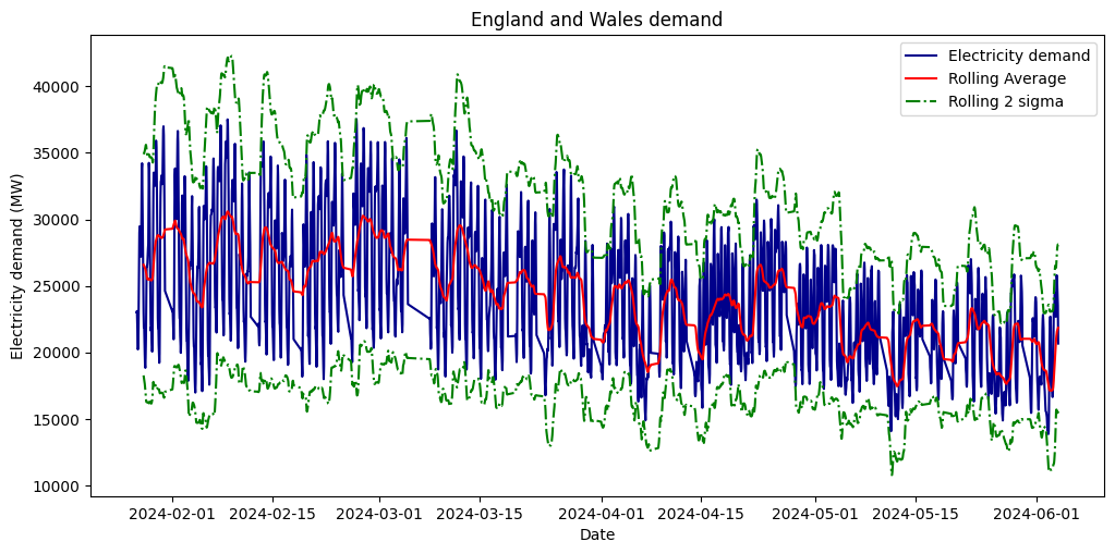
The above image shows the electricity demand in England and Wales, the one day rolling average and the one week rolling 2 sigma curves.
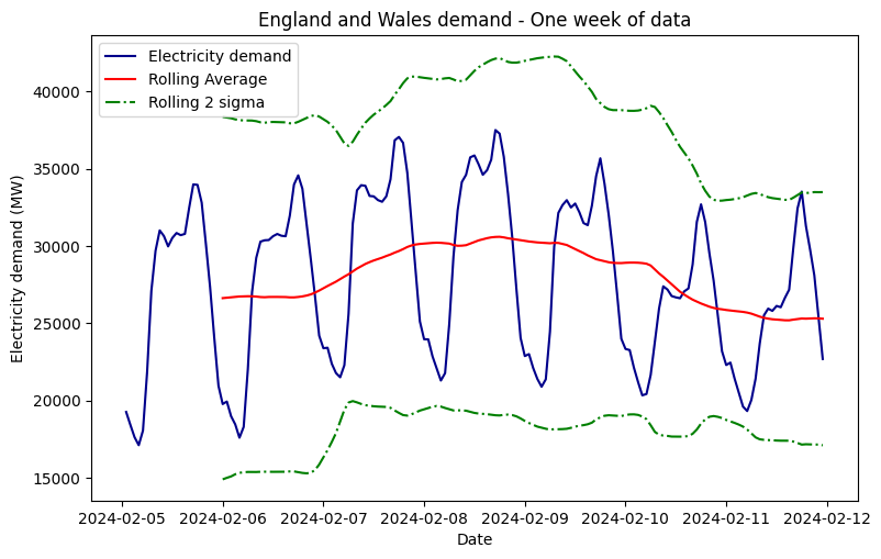
Something that stands out in the previous images is the parts of the plot where there's a straight line connecting sampled from different days. That corresponds to missing values. In order to keep the daily seasonality, which can be seen in the next plot, I removed the data for those days where there is at least one missing sample. In order to observe the daily pattern, one can zoom in and focus on just one week:
In order to keep this section brief, the reader is encouraged to check the Jupyter notebook to find out more about the decomposition into trend, seasonality and residuals. Since ARIMA model won't be used, these parameters aren't that relevant.
Also, the Kaggle notebook helped me gain more insight about the data since I could use the electricity demand from 2009 to 2024 (in case you wonder why I'm not using it for this project, it's because the weather data is only available from 26/01/2024):
- There's weekly seasonality and yearly seasonality in the data
- Bank holidays affect the energy consumption
- Electricity consumption is lower during summer
- Electricity consumption is trending down. In 2009, the average electricity consumption (for TSD, not just England and Wales) was around 38,000 MW per hour, whereas in 2023 the average electricity consumption was 28,000 MW per hour
Prototyping
Before talking about the models, it is necessary to define the metrics that will be used to assess the performance:
- R-square
- Mean Square Error (MSE)
- Root Mean Square Error (RMSE)
- Mean Absolute Error (MAE)
- Mean Absolute Percentage Error (MAPE)
In the Planning section section I mentioned the models I used in my previous project on electricity demand forecasting. For this project, I considered the following models:
- XGBoost
- Linear Tree
- Linear Boosting
All of these algorithms meet some of the requirements of the prediction service: they're fast to train on CPU.
Beyond finding what the best performing model, I wanted to test whether adding weather data led to more accurate predictions. In my original project, I only used the past data and features such as the day of the week and month of the year to train the model. Adding weather data leads to a more complex infrastructure, but the extra complexity is worth it if it leads to more accurate predictions.
Evaluation
The goal of running the experiments was to:
- Find out what model yields the best results with minimal hyperparameter tunning (proper hyperparameter tunning will be performed at a later stage)
- Find out if adding weather data improves the predictions
The results are summarised by the following table:
| Model | MAE | MAPE | MSE | RMSE | Explained Var | R2 |
|---|---|---|---|---|---|---|
| xgb_simple | 2292.5 | 11.6 | 7892710.0 | 2809.4 | 0.7 | 0.3 |
| xgb_advanced | 2302.6 | 11.7 | 7976893.0 | 2824.3 | 0.8 | 0.3 |
| linear_boost_simple | 2295.6 | 11.3 | 8080621.0 | 2842.6 | 0.4 | 0.3 |
| linear_boost_advanced | 3291.8 | 16.6 | 15724100.0 | 3965.4 | 0.2 | -0.3 |
| linear_trees_simple | 1563.8 | 7.5 | 4059538.0 | 2014.8 | 0.7 | 0.7 |
| linear_trees_advanced | 1551.7 | 7.5 | 4014264.0 | 2003.6 | 0.7 | 0.7 |
| xgb_simple - no weather | 2992.0 | 15.1 | 12084520.0 | 3476.3 | 0.7 | -0.0 |
| xgb_advanced - no weather | 3377.8 | 16.9 | 14913750.0 | 3861.8 | 0.7 | -0.3 |
| linear_boost_simple - no weather | 2107.2 | 10.6 | 7109882.0 | 2666.4 | 0.5 | 0.4 |
| linear_boost_advanced - no weather | 4049.6 | 20.7 | 57325420.0 | 7571.4 | -3.3 | -3.9 |
Note that the difference between simple and advanced models is simply increasing the values of a few hyperparameters. Proper hyperparameter tuning will be performed as part of the MVP.
The above dataframe, which is used as a summary table, shows that:
- Linear trees are the best performing model, both in its simple and advanced versions. An added bonus is that is the second fastest model to train after XGBoost.
- Using weather data leads to be better results
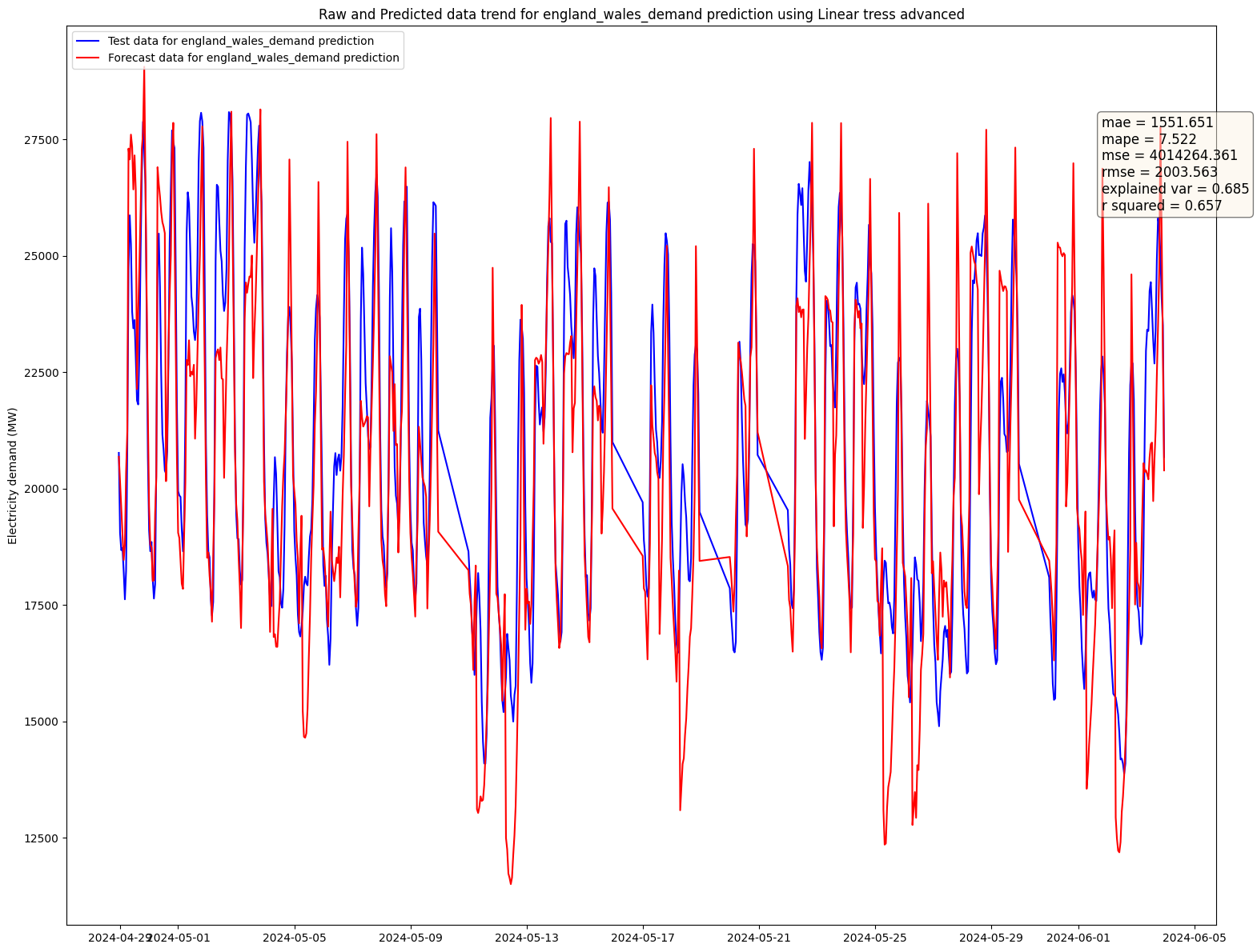
The comparison of the linear trees model with the test data is as follows:
Before, wrapping up model experimentation. I would like to address some of the questions that Ben Wilson includes at the end of chapter 6 (the rest of the questions aren't that relevant for this project as this project isn't meant to create a proprietary prediction service):
-
How often does this need to run? (The question actually refers to training and not inference)
- The model will be re-trained daily until a stable model is found. After that, the model will only be re-trained when the performance drops beyond a given threshold
-
Where is the data for this right now?
- Data is available right now. Electricity demand data is available at any time and the weather data is fetched, updated and stored daily.
-
Where are the forecast going to be stored?
- The model will be accessed through an API and web app will be available to visualise some dashboards. The tool to store the forecasts hasn't been decided yet, but it needs to fulfill these needs.
-
Where is this going to run for training?
- Once past the MVP stage, the project will be deployed to a server where the training will be run.
-
Where is the inference going to run?
- Same as above, in a server
-
How are we going to get the predictions to the end users?
- Via API